Image processing, pt 1 - NL-BioImaging Advanced Image Analysis Course 2026

Martijn Wehrens, Bram van den Broek (version: 0.9)

Libraries¶

Libraries are packages of code that people have written, and can be loaded.

We’ll be using code for plotting, importing files, and image analysis.

# Plotting libraries
import matplotlib.pyplot as plt
import seaborn as sns
# Library to load tiff files
import tifffile as tiff
# General math libraries
import numpy as np
from scipy import stats
# Image analysis libraries/modules
import skimage as sk
from scipy import ndimage

Segmentation and thresholding¶

A computer doesn’t “know” what biological features are, unless we explicitly program it. For example, if we want to analyze cells, we’ll need to be able to create a computer program that first of all knows which of the pixel of an image belong to a (single) cell.

Creating such regions of interest (ROIs) in an image is called segmentation.

Case 1: segmenting an image with bimodal intensity profile¶

# Load the image using tiff library
img_happycell = tiff.imread("images/happy_cell_noise.tif")

_ = plt.imshow(img_happycell)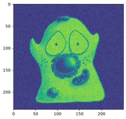

# Show the histogram
_ = plt.hist(img_happycell.ravel(), bins=256)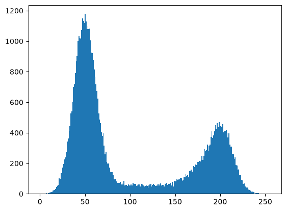



# Create a figure to display the image and it's histogram
fig, axs = plt.subplots(1,2, figsize=(10/2.54, 5/2.54))
_ = axs[0].imshow(img_happycell)
_ = axs[0].set_xlabel("pixels")
_ = axs[0].set_ylabel("pixels")
_ = axs[1].hist(img_happycell.ravel(), bins=256)
_ = axs[1].set_xlabel("Intensity")
_ = axs[1].set_ylabel("Counts")
_ = plt.tight_layout()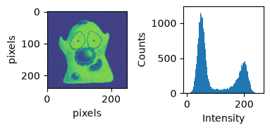

<Figure size 393.701x196.85 with 2 Axes>

The intensity distribution of this image is called “bimodal”, since it has two peaks.

Intermezzo: using functions¶

# To avoid re-writing code, create a function that does the same
def plot_img_and_hist(img):
    
    """Create a figure to display the image and it's histogram"""
    
    fig, axs = plt.subplots(1,2, figsize=(15/2.54, 5/2.54))
    # Plot image
    _ = axs[0].imshow(img)
    _ = axs[0].set_xlabel("pixels")
    _ = axs[0].set_ylabel("pixels")
    # Plot histogram
    _ = axs[1].hist(img.ravel(), bins=256)
    _ = axs[1].set_xlabel("Intensity")
    _ = axs[1].set_ylabel("Counts")
    _ = plt.tight_layout()

    return fig, axs

# And now call that function to test it
_, _ = plot_img_and_hist(img_happycell)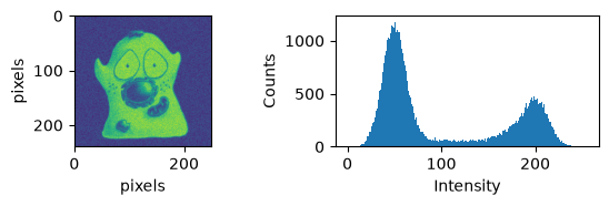

<Figure size 590.551x196.85 with 2 Axes>

# A function is a piece of code that you can run by 
# typing the function name.
# It has inputs (arguments), and an output (return value).

# Function definition, the arguments, which you 
# can freely name, are between round brackets
def add_ab(a, b):
    # Documentation can go between three quotes.
    """ Return the sum of a and b. """

    # Some code
    c = a + b

    # Say what should be returned
    return c

# Now the function can be "called" by it's name, and it 
# will "return" the chosen values.
add_ab(2, 5)

7

Source materials: img_happycell is taken from biobook (fig. 68), Creative Commons Attribution 4.0 International License.

The segmentation¶

One algorithm that works well on bimodal distributions is Otsu’s method. It will try to find a threshold that minimizes the variance in the intensities that respectively fall above and below that threshold. (For more info, see biobook.)

# Call the function to determine the otsu threshold from scikit image
thresh_otsu = sk.filters.threshold_otsu(img_happycell)
# Plot the result
fig, axs = plot_img_and_hist(img_happycell)
_ = axs[1].axvline(thresh_otsu, color="red")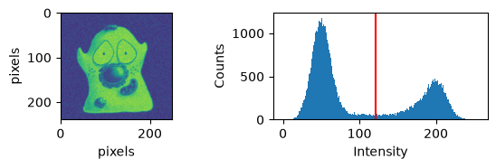

# We can create a "mask", a binary image that represent 
# foreground and background
mask_happycell = img_happycell>thresh_otsu
# Inspecting what we did
mask_happycell[50:100, 50:100]

array([[False, False, False, ...,  True,  True,  True],
       [False, False, False, ...,  True,  True,  True],
       [False, False, False, ...,  True,  True,  True],
       ...,
       [ True,  True,  True, ...,  True,  True,  True],
       [ True,  True,  True, ...,  True,  True,  True],
       [ True,  True,  True, ...,  True,  True,  True]], shape=(50, 50))

_ = plt.imshow(mask_happycell)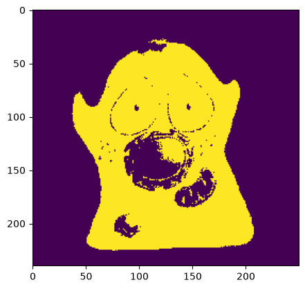

Case 2: segmenting an image with a dominant background¶

# Load image with kinase translocation reporter data
# Channel 0 are nuclei
img_nuclei = tiff.imread("images/KTR_t0.tif")[0,:,:]

# display
fig, axs = plot_img_and_hist(img_nuclei)
axs[1].set_yscale("log") # (not everyone likes this)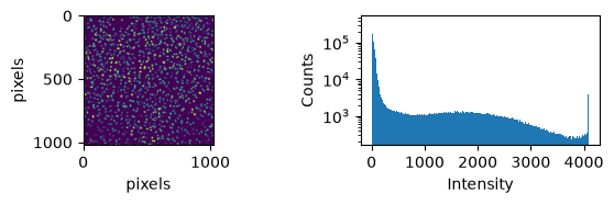

As can be seen, this image doesn’t have a bimodal distribution, intead, it has a very strong background peak, and a relatively small number of pixels with higher intensity.

In this image, we’ll aim to identify pixels that are above the dominant background peak.

Methodology¶

A method that’s suitable for the “dominant background” case is the “triangle method”, which was published already by Zack et al. in 1977.

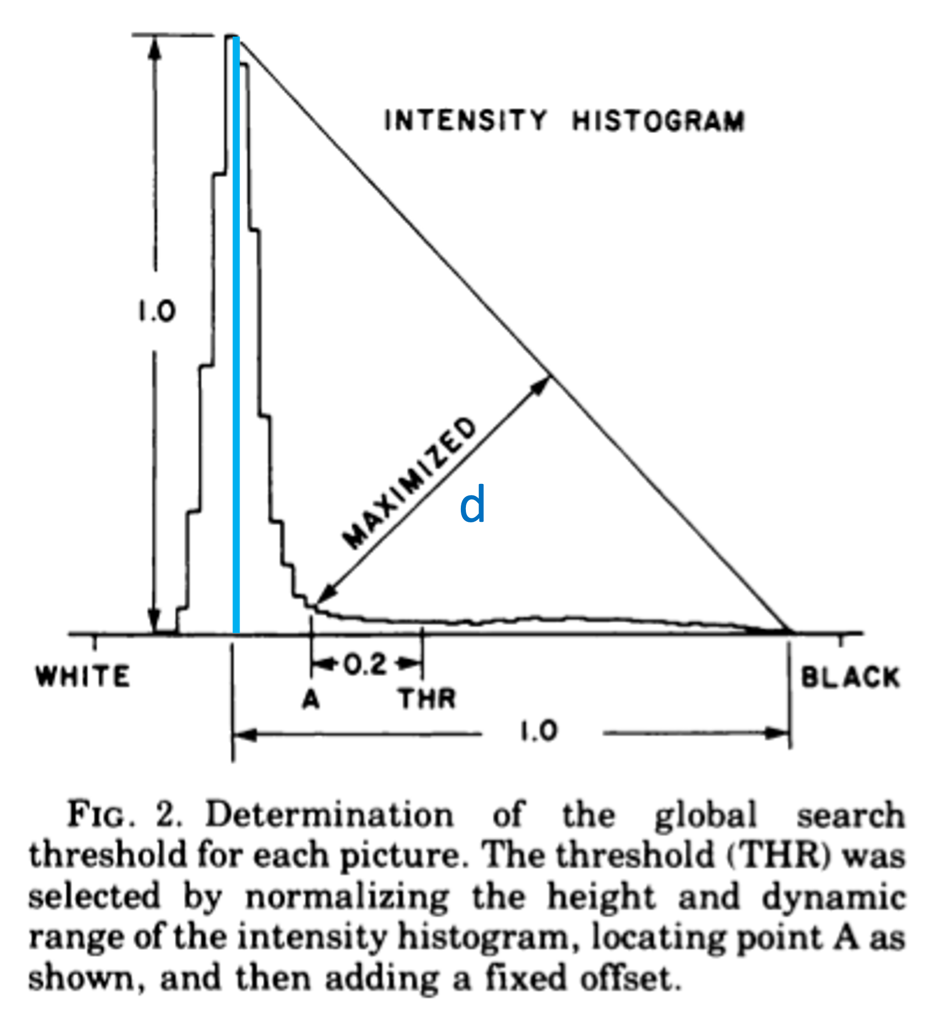
In the figure above (from Zack et al.), the method is explained. A line is drawn in the histogram between $x_\text{mode}, y(x_\text{mode})$ and $x_\text{max}, 0$ . Then, a second line is drawn, perpendicular to the first line, which maximizes the distance to the histogram line. The x-value where that second line touches the histogram, will be the threshold. (Originally, a margin of 0.2 was included, but modern implementations leave that out.)

# Apply the triangle method
thresh_triangle = sk.filters.threshold_triangle(img_nuclei)
mask_nuclei = img_nuclei > thresh_triangle

fig, axs = plot_img_and_hist(img_nuclei)
axs[1].axvline(thresh_otsu, color="red")
axs[1].set_yscale("log")
thresh_otsu

np.int64(121)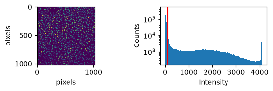

plt.imshow(mask_nuclei)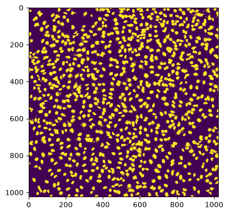

More thresholding-finding algorithms¶

More thresholding-finding algorithms exits. Threshold methods included in skimage.filters are:

threshold_isodata()
threshold_li()
threshold_mean()
threshold_minimum()
threshold_multiotsu()
threshold_niblack()
threshold_otsu()
threshold_sauvola()
threshold_triangle()
threshold_yen()

Local thresholding¶

What we’ve seen so far are single threshold values that we apply to the whole image, ie “globally”. These are therefor global thresholds.

Let’s look at an example where this goes wrong.

# Another example image
img_page = tiff.imread("images/page_original.tif")
plot_img_and_hist(img_page)

(<Figure size 590.551x196.85 with 2 Axes>,
 array([<Axes: xlabel='pixels', ylabel='pixels'>,
        <Axes: xlabel='Intensity', ylabel='Counts'>], dtype=object))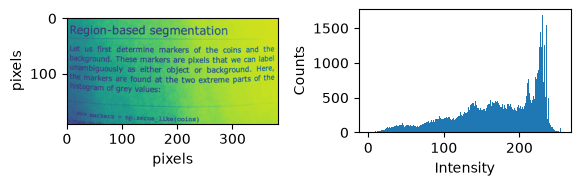

# When text is foreground, invert the image
img_page_inverted = np.invert(img_page)
_, _ = plot_img_and_hist(img_page_inverted)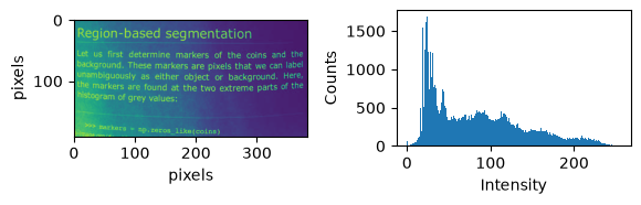

# Apply triangle
threshold_page1 = sk.filters.threshold_triangle(img_page_inverted)
mask_triangle = img_page_inverted > threshold_page1
_ = plt.imshow(mask_triangle)

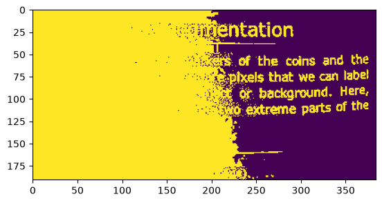
However, if we inspect parts of the image separately, we might be able to find thresholds that can be applied locally that do separate back- and foreground.

# Find local threshold, i.e. for each pixel separately
# This will thus generate an array of size equal to the image
thresh_local = \
    sk.filters.threshold_local(
        img_page_inverted, 
        block_size=35, # check a "neighborhood" of 35x35 around each pixel
        offset=-10 # adjust the per-pixel thresholds globally by subtracting this number
    )

# Inspect shape (two methods)
print(np.shape(thresh_local))
print(thresh_local.shape)
# Show the result
print(thresh_local[1:10,1:10])

(191, 384)
(191, 384)
[[130.77211822 130.90207039 131.08406619 131.3037651  131.54411986
  131.78670404 132.01305378 132.20621863 132.35203808]
 [131.05212856 131.19449961 131.39410716 131.63543722 131.89996679
  132.16758333 132.41804769 132.63270539 132.7958992 ]
 [131.46965599 131.6316074  131.85895878 132.13432677 132.43684833
  132.74375233 133.03201741 133.2803335  133.47072804]
 [132.02108962 132.21072415 132.47726401 132.80065482 133.15670758
  133.51889678 133.86029997 134.15590792 134.38455086]
 [132.70090606 132.92728526 133.24579583 133.63280466 134.05969015
  134.49495656 134.90655574 135.2646515  135.54394112]
 [133.50142723 133.77439631 134.15875392 134.62629676 135.14277097
  135.67040636 136.17073221 136.60790608 136.9515313 ]
 [134.41221196 134.74198931 135.2065921  135.77222055 136.39775503
  137.03782359 137.64623024 138.17995689 138.60257775]
 [135.41969318 135.81625928 136.37517213 137.05604269 137.80970077
  138.58191197 139.31753654 139.96530408 140.4819182 ]
 [136.50676645 136.97913384 137.64506655 138.45670846 139.3557997
  140.27815383 141.15865687 141.93689572 142.5620314 ]]

# Create a mask
mask_page = img_page_inverted>thresh_local
plt.imshow(mask_page)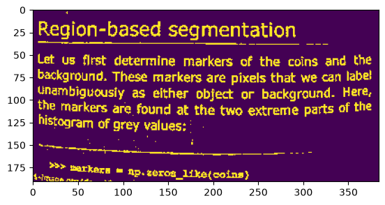

Exercise: thresholding bacteria¶

Can you apply some of the above methods to the image loaded below? We’ll discuss in 5-10 minutes.

img_ecoli = np.invert(tiff.imread('images/microcolony_ecoli.tif'))
_, _ = plot_img_and_hist(img_ecoli)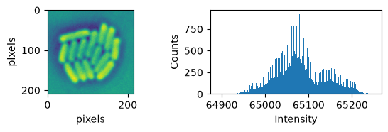

More advanced image processing¶

For the example above, and many biological images, features are not straightforward to extract. We need more advanced methods than simple thresholding.

We’ll introduce you to some advanced image processing methods, and apply them later to biological examples.

Convolution¶

Convolutational image operations are at the heart of many image processing steps. You’ll also see them a load in machine learning.

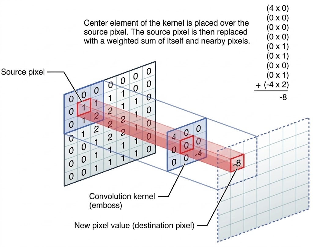
Image source: via discuss.pytorch.org.

In convolution, a new image of equal size is created. The procedure goes over each pixel $(i, j)$ in the original image, and sums its neighborhood pixels multiplied with neighborhood location specific weights, to get the intensity value for the new pixel at location $(i ,j)$ .

This allows you to manipulate the image in very useful ways.

Examples (1)¶

# Let's illustrate this concept with some examples

# Load an example picture
img_pika = tiff.imread('images/pikachu.tif')
_= plt.imshow(img_pika)
_= plt.colorbar()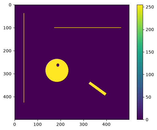

# Define a horizontal line "kernel"
kernel_h = np.zeros((25,25))
kernel_h[12,:] = 1
kernel_h=kernel_h/np.sum(kernel_h)
plt.imshow(kernel_h)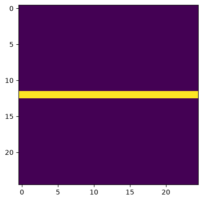

# Define a vertical line "kernel"
kernel_v = np.zeros((25,25))
kernel_v[:,12] = 1
kernel_v=kernel_v/np.sum(kernel_v)
plt.imshow(kernel_v)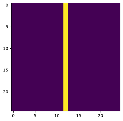

# Apply them both to the image
img_pika_h = ndimage.convolve(img_pika, kernel_h)
img_pika_v = ndimage.convolve(img_pika, kernel_v)

# Now show both pictures
fig, axs = plt.subplots(1,2)
axs[0].imshow(img_pika_h, cmap='magma')
axs[1].imshow(img_pika_v, cmap='magma')
plt.show()

# Can you see what happened?
    # shapes
    # intensities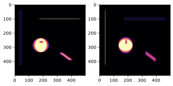

Do you understand why the results looks like it does? Both how the shapes have changed, and also how the intensities have changed?

Examples (2)¶

# Define a disk kernel
kernel_disk = sk.morphology.disk(15) 
kernel_disk = kernel_disk/np.sum(kernel_disk)
_ = plt.imshow(kernel_disk)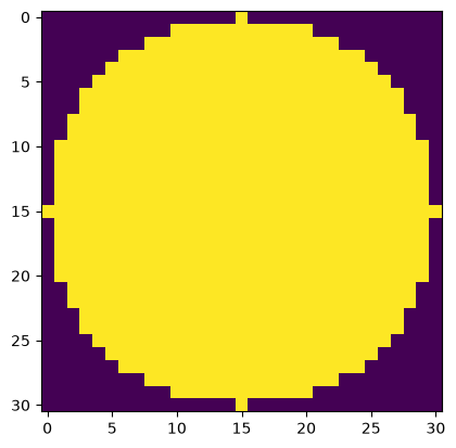

# Define an edge kernel
kernel_laplacian = np.array(
    [[0, -1,  0],
     [-1,  4, -1],
     [0, -1,  0]])

# Now apply and plot
img_pika_disk = ndimage.convolve(
    img_pika.astype(np.float32), 
    kernel_disk.astype(np.float32)
    )
img_pika_edge = ndimage.convolve(
    img_pika.astype(np.float32), 
    kernel_laplacian.astype(np.float32)
    )
minmaxval1 = np.max(np.abs(img_pika_disk))
_ = plt.imshow(img_pika_disk, cmap='seismic', vmin=-minmaxval1, vmax=minmaxval1)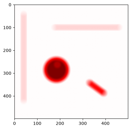

minmaxval2 = np.max(np.abs(img_pika_edge))
_ = plt.imshow(img_pika_edge, cmap='seismic', vmin=-minmaxval2, vmax=minmaxval2)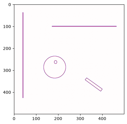

The seismic colormap, when centered around 0, shows positive values in red, and negative values in blue.

The first image looks blurred, and in the second image edge structures remain.

Do you understand why the 1st image is blurred? Why edges remain in the second image are a bit more complicated. Can you take a guess as to why this is?

The laplacian¶

We’ll skip the math here, but the “laplacian” kernel equals a pixel’s 2nd derivative. The image below illustrates why that helps to detect sudden intensity changes.

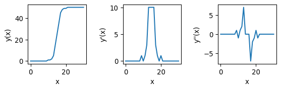
The left panel shows an intensity change in one dimension, here $y$ would be the intensity and $x$ the location along the image. The middle panel shows that the derivative peaks at the “edge” (note that the peak would be negative if the change goes in the other direction). The right panel shows that around the edge, the double derivative first shows a positive peak and then a negative peak.

Thus, in the second derivative image, pixels that are near-zero and which are in the vicinity of both a negative and positive value, are close to an edge.

Technical note¶

Both the derivative and laplacian kernel can be used to find edges. The advantage of the Laplacian is that it better identifies the exact location of the edge, as the zero-crossing (pixels with values close to zero) are precisely where the edge is. First-order derivatives can also be used, but they are dimension-specific (either the derivative in the row-direction, or the derivative in the column-direction), so the output of two convolutions needs to be combined. Additionally, both can be sensitive to noise, why they are often combined with a de-noising convolution (e.g. blur), as we will see below.

Dilation and erosion¶

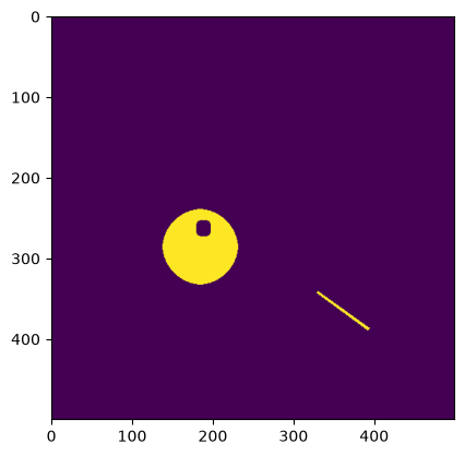
As we’ll see, it is often convenient to manipulate binary masks.

Morphological operations, similar to the convolution, also construct a new picture on a pixel-by-pixel basis. They look at properties of the set of neighborhood intensity values.

The main operations are:

Dilation, which takes the neighborhood maximum.
Erosion, which takes the neighborhood minimum.

# Let's try
img_pika_eroded  = sk.morphology.erosion(img_pika, footprint=np.ones((7,7)))
plt.imshow(img_pika_eroded)


img_pika_dilated = sk.morphology.dilation(img_pika, footprint=np.ones((7,7)))
plt.imshow(img_pika_dilated)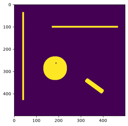

Combining operations¶

These operations can also be applied to grayscale images.

There exist multiple combinations of morphological operations that are often used together, such as:

Opening (erode → dilate): removes small features, keeps coarse features.
Closing (dilate → erode): fills small holes/gaps.
Top-hat (image − opening): isolates small bright features (background-subtraction, spot-detection)
Morphological gradient (dilation − erosion): edges.

Exercise: Apply opening and closing¶

Apply sk.morphology.closing and sk.morphology.opening to the “pikachu” image. Do you understand the result?
Use the argument footprint=sk.morphology.disk(7). Does this change the outcome? Why?

We’ll discuss in 5-10 minutes.

Built-in filtering and edge detection¶

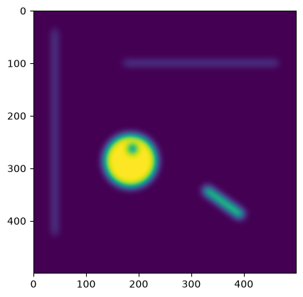
With the above tools, we could make custom functions that perform edge detection or blurring.

There are however also some optimized built-in functions that perform these tasks.

# Blurring using a Gaussian kernel
img_pika_gauss07 = sk.filters.gaussian(img_pika, sigma=7)
_ = plt.imshow(img_pika_gauss07)

# Stronger blur
img_pika_gauss20 = sk.filters.gaussian(img_pika, sigma=20)
_ = plt.imshow(img_pika_gauss20)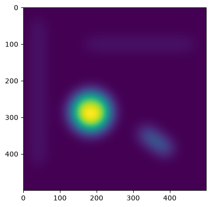

Edge detection methods¶

There exist multiple built-in edge detection methods, common ones include: sk.filters.sobel(), sk.filters.prewitt(), sk.filters.laplace(), sk.feature.canny(). See also the documentation.

# Let's try Sobel on the nuclei
img_edges = sk.filters.sobel(img_nuclei)
_ = plt.imshow(img_edges[0:200,0:200]) # e.g. threshold > 0.01, or use local threshold?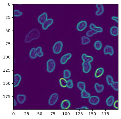

Neighborhood-based filtering¶

Neighborhood-based filtering methods include ndimage.minimum_filter(), ndimage.maximum_filter, ndimage.median_filter().

The median filter is for example relevant to remove noise from images.

img_noisy = tiff.imread("images/spots.tif")
plot_img_and_hist(img_noisy)

(<Figure size 590.551x196.85 with 2 Axes>,
 array([<Axes: xlabel='pixels', ylabel='pixels'>,
        <Axes: xlabel='Intensity', ylabel='Counts'>], dtype=object))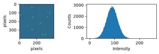

img_noisy_median = ndimage.median_filter(img_noisy, footprint=sk.morphology.disk(4))
fig, axs = plot_img_and_hist(img_noisy_median)
axs[1].set_yscale("log")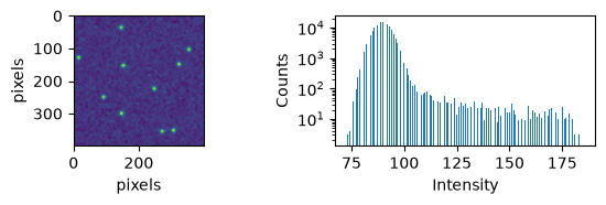

Exercise: thresholding¶

Can you create a binary mask for the points in img_noisy?
Can you create a binary mask that contains the edges of img_nuclei?

Optional help: hints for the nuclear edges¶

One solution involves using a combination of erosion(), the original nuclei_mask, and combining different masks using np.logical_..() (documentation).

If you want a polished result, perhaps you can also throw in an opening() operation.

References¶

Zack, G. W., Rogers, W. E., & Latt, S. A. (1977). Automatic measurement of sister chromatid exchange frequency. Journal of Histochemistry & Cytochemistry, 25(7), 741–753. 10.1177/25.7.70454