Image processing, pt 3/3 - NL-BioImaging Advanced Image Analysis Course 2026

# Libraries

# Plotting libraries
import matplotlib.pyplot as plt
import seaborn as sns
# Library to load tiff files
import tifffile as tiff
# General math libraries
import numpy as np
from scipy import stats
# Image analysis libraries/modules
import skimage as sk
from scipy import ndimage
# Data handling
import pandas as pd

Combining multiple operations¶

Let’s load the bacterial data again:

img_ecoli = np.invert(tiff.imread('images/microcolony_ecoli.tif'))
_ = plt.imshow(img_ecoli)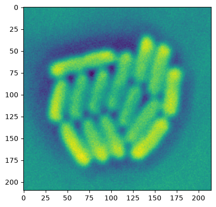

Some (many) image features cannot be captured by application of a single image processing function.

By combining several image processing tools however, you can sometimes extract more complex features.

Let’s look at an example of this: a multi-step approach allows us to segment the bacterial picture we saw before.

#### Laplacian + Gauss

# Combination of these is a good edge detector

# Apply of LoG on the bacteria
img_ecoli_gauss = sk.filters.gaussian(img_ecoli, sigma=3)
edges_log = sk.filters.laplace(img_ecoli_gauss)

# show both
_ = plt.title("After Gauss")
_ = plt.imshow(img_ecoli_gauss)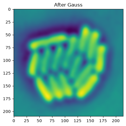


minmaxval = np.max(np.abs(edges_log))
_ = plt.title("After Gauss & Laplacian")
_ = plt.imshow(edges_log, cmap='seismic', vmin=-minmaxval, vmax=minmaxval)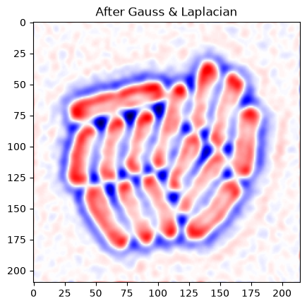

As we saw earlier, edges correspond to values going from positive, through zero, to negative. So we can look for places where negative and positive values are close.

# Now identify edge pixels
    # where value goes positive->negative (or vice versa)
    # ie positive and negative value close
    #
    # (Technical note: e.g. Matlab has a built-in function 
    # edge detection function based on the LoG, in Python, 
    # we need to custom-code this.)

# per pixel, what's lowest and highest neighbor
edges_min = ndimage.minimum_filter(edges_log, footprint=sk.morphology.disk(1))
edges_pos = ndimage.maximum_filter(edges_log, footprint=sk.morphology.disk(1))
# do we find both positive & negative close?
img_edges = np.logical_and(edges_min < 0, edges_pos >0)

plt.imshow(img_edges)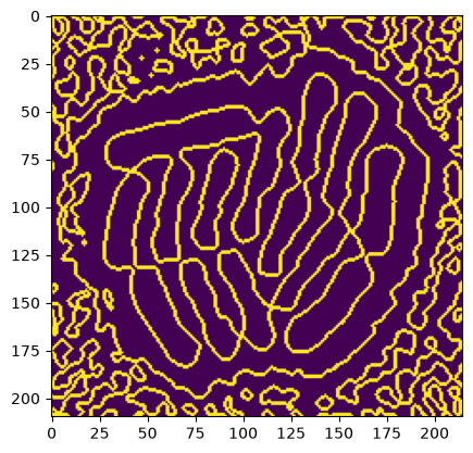

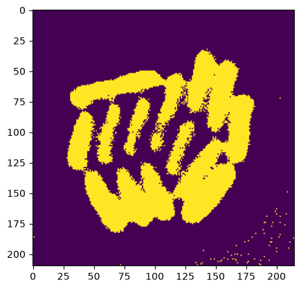
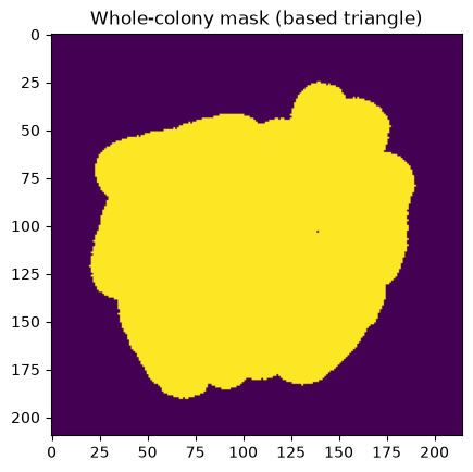
Let’s remove lines due to background noise by using a simpler triangle mask to select the colony.


# Use previous thresholded image 
    # Make whole-colony mask    
mask_ecoli_triangle = img_ecoli > sk.filters.threshold_triangle(img_ecoli)

_ = plt.imshow(mask_ecoli_triangle)

# Modify this mask

# Remove small parts
mask_ecoli_triangle_filtered = \
    sk.morphology.remove_small_objects(
        mask_ecoli_triangle, 
        max_size=50
    )
# Enlarge it
mask_ecoli_triangle_filtered = \
    sk.morphology.dilation(
        mask_ecoli_triangle_filtered, 
        footprint=sk.morphology.disk(8)
    )

_ = plt.title("Whole-colony mask (based triangle)")
_ = plt.imshow(mask_ecoli_triangle_filtered)

# Combine both
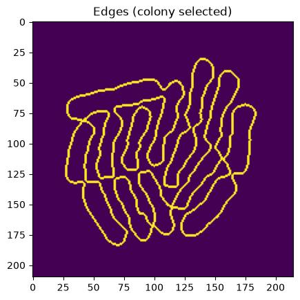
img_edges_foreground = np.logical_and(img_edges, mask_ecoli_triangle_filtered)
_ = plt.title("Edges (colony selected)")
_ = plt.imshow(img_edges_foreground)

# And fill outlines
img_edges_filled = ndimage.binary_fill_holes(img_edges_foreground)
_ = plt.title("Segmented bacteria (v1)")
_ = plt.imshow(img_edges_filled)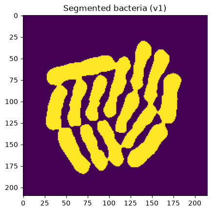

This looks pretty great, except that many bacteria are still “stuck together”.

Let’s try to identify separate bacteria.

# Let's erode this by 4 px
# (Aim: get indivdual bacterial locations)
mask_ecoli_log_eroded = \
    sk.morphology.erosion(
        img_edges_filled, 
        footprint=sk.morphology.disk(4)
    )

# Show
_ = plt.imshow(mask_ecoli_log_eroded, cmap='gray')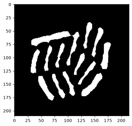

# And label
mask_bacteria_slim_labeled = sk.measure.label(mask_ecoli_log_eroded)
_ = plt.imshow(mask_bacteria_slim_labeled, cmap='tab20')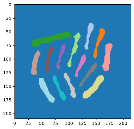

We can now combine the “shrunk” but individually separated bacteria with the original binary mask, to obtain individually separated bacteria in the proper bacterial mask.

To achieve this, we’ll use a function we haven’t seen yet, which is called “watershed”.

This “fills” an image intensity profile with “water” at separate marker locations designated by a labeled map. As the global waterlevel rises, wherever water starts touching, region boundaries are set.

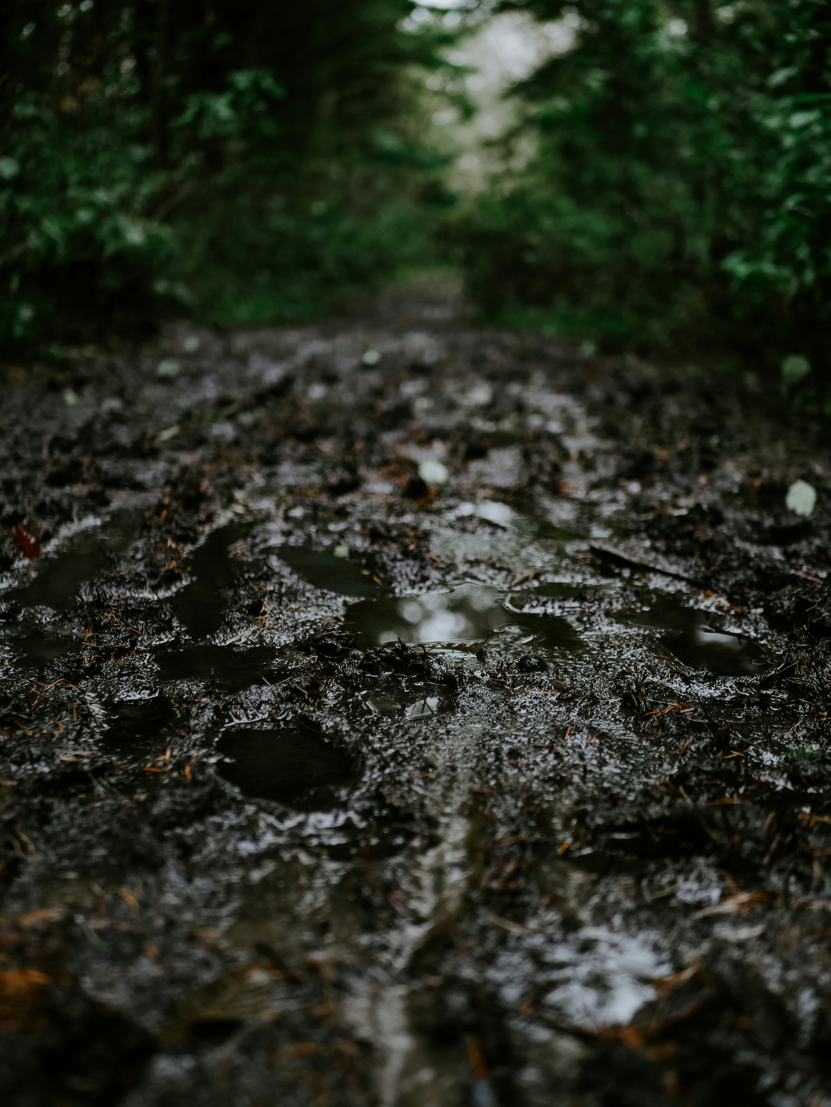
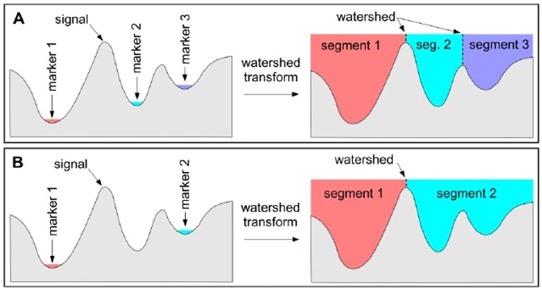
(Pictures via Matt Seymour on Unsplash and researchgate.) Watershed is a common algorithm to segment touching objects. It is inspired by how water would fill up a landscape. From specific seeds, the water level rises, and once separate regions touch, boundaries are established.

# Apply to separate bacteria
    # Using mask_ecoli_log
    # mask_bacteria_slim_labeled as seeds
mask_bacteria_combined = \
    sk.segmentation.watershed(
        -1*img_edges_filled, 
        markers=mask_bacteria_slim_labeled, 
        mask=img_edges_filled
    )

# Show the result
_ = plt.title("Segmented individual bacteria")
_ = plt.imshow(mask_bacteria_combined, cmap='viridis')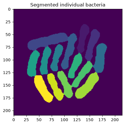

Great! We now have a labeled map where we can access information about each of the single bacteria that were recorded.

# Polish the final image a little bit

# Let's get regionprops from mask_bacteria_combined
props = sk.measure.regionprops(mask_bacteria_combined)

# Plot it
fig, ax = plt.subplots(1,1, figsize=(9/2.54,9/2.54))
_ = ax.imshow(img_ecoli, cmap='gray')
# slightly shaded region
# plt.imshow(mask_bacteria_combined, cmap='jet', alpha= .3*(mask_bacteria_combined>0))
# project numbered labels on top
for x,y,lbl in [(p.centroid[1], p.centroid[0], p.label) for p in props]:
    # centered text
    ax.text(x, y, str(lbl), color='white', fontsize=9, ha='center', va='center')
    # specific bacterial outline
    ax.contour(mask_bacteria_combined==lbl, colors='red', linewidths=0.5)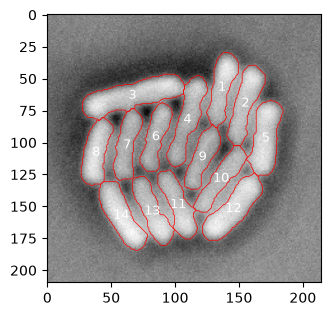

<Figure size 354.331x354.331 with 1 Axes>

Exercise: Batch analysis of the KTR data¶

Download the file KTR-images-series.zip (link), which contains the following folders:
- sensor/
  - KTR_sensor_frame_0000.tif
  - KTR_sensor_frame_0001.tif
  - (..)
- nuclei/
  - KTR_nuclei_frame_0000.tif
  - KTR_nuclei_frame_0001.tif
  - (..)
Use a loop to load these images into one big np.array().
Write a function that calculates the KTR C/N ratio, like we did in part 2
- The function should take as input arguments img_nuclei and img_KTR, respectively data from a single frame of nuclei or KTR sensor image data.
- The function should then return all C/N ratios from that image per cell in a single array.
Use a loop to apply this function to all time points of the data.
Plot the data

Notes: Time between frames is 270.01617 seconds. Stimulation occured at 25 mins.

Hints¶

The following generic structure can be used to loop over files and load them:

for t in range(nr_frames):
    img = tiff.imread(<path> + str(t).zfill(4) + ".tif")

With my_list = [] you can start an array
With the command my_list.append(img) you can add items (likely images in this case) to an array (also when it’s empty).
np.array(my_list) can convert a list to a numpy array.
When making a plot, a loop can be used to plot different parts of the data. E.g.:

for t in range(nr_frames):
    _ = plt.scatter(<x values>, <y values for t>)

The code [t]*100 creates an array of length 100 in which the value of t is repeated.
len(my_list) gives the length of a list.

References¶

Fisher, A. (2014). Cloud and Cloud-Shadow Detection in SPOT5 HRG Imagery with Automated Morphological Feature Extraction. Remote Sensing, 6(1), 776–800. 10.3390/rs6010776