Deep learning for segmentation: StarDist - NL-BioImaging Advanced Image Analysis Course 2026

This notebook is inspired by StarDist prediction example notebook.

StarDist is a neural network that predicts for every pixel how likely it is to be the centre of an object and what the shape of that object is. The shape is described as a star-convex polygon: rays going from the centre outwards to the boundary. Because a shape is predicted per object, touching nuclei come out as separate objects. This is what is called instance segmentation.

We use a pretrained StarDist model: the network was already trained on many annotated nuclei, and we only run the prediction from the model.

Libraries¶

# We import the necessary libraries for plotting and image reading and processing
import matplotlib.pyplot as plt
import tifffile as tiff
import numpy as np
import skimage as sk

# We import StarDist, and the normalization helper from csbdeep, a related library for deep learning in microscopy
from stardist.models import StarDist2D
from stardist import random_label_cmap
from csbdeep.utils import normalize

# Colormap that gives every label a different random color
lbl_cmap = random_label_cmap()

Test on example data¶

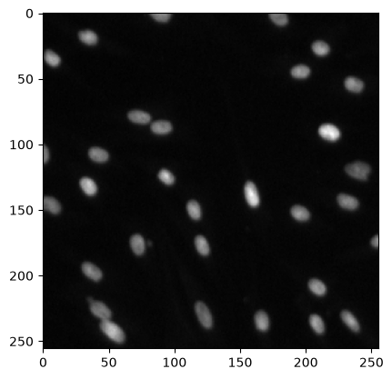
We start with an image from the dataset the model was trained on (DSB2018, a collection of annotated nuclei). We use it first, before trying some other images.

img_dsb = tiff.imread("data/stardist_example1.tif")
print(img_dsb.shape, img_dsb.dtype)

_ = plt.imshow(img_dsb, cmap="gray")

(256, 256) uint8

Loading a pretrained model¶

StarDist ships with a few pretrained models. Calling from_pretrained() without arguments prints the list.

# Show which pretrained models are available
StarDist2D.from_pretrained()

There are 4 registered models for 'StarDist2D':

Name                  Alias(es)
────                  ─────────
'2D_versatile_fluo'   'Versatile (fluorescent nuclei)'
'2D_versatile_he'     'Versatile (H&E nuclei)'
'2D_paper_dsb2018'    'DSB 2018 (from StarDist 2D paper)'
'2D_demo'             None

We pick the 2D_versatile_fluo model, which is trained on a variety of fluorescent images. It will download the model from the internet if it is not already present on your computer.

model = StarDist2D.from_pretrained("2D_versatile_fluo")

Found model '2D_versatile_fluo' for 'StarDist2D'.
Loading network weights from 'weights_best.h5'.
Loading thresholds from 'thresholds.json'.
Using default values: prob_thresh=0.479071, nms_thresh=0.3.

# Only if you get an error above on Windows uncomment this and run it once to copy the model files to a location where they can be found

#import shutil, tempfile
#from pathlib import Path

#for base in [Path.home() / ".keras", Path(tempfile.gettempdir()) / ".keras"]:
#    d = base / "models" / "StarDist2D" / "2D_versatile_fluo"
#    src, dst = d / "2D_versatile_fluo_extracted", d / "2D_versatile_fluo"
#    if src.is_dir() and not dst.exists():
#        shutil.copytree(src, dst)
#        print("copied to", dst)

Normalization¶

The network was trained on images whose intensities were scaled between 0-1. If we feed it raw microscope images, which are either 0-255 for 8-bit or 0-65535 for a 16-bit image the numbers are far outside the range the model has ever seen, and the predictions get worse.

We run a normalization function to scale the image between 0 and 1. normalize(img, 1, 99.8) sets the 1st percentile of the intensities to 0 and the 99.8th percentile to 1. We use percentiles instead of the minimum and maximum so that a handful of bright pixels do not affect the normalization. The values are not clipped, so the brightest pixels end up slightly above 1.

img_dsb_norm = normalize(img_dsb, 1, 99.8)

print(f"before normalization: {img_dsb.min()} to {img_dsb.max()}: type {img_dsb.dtype}")
print(f"after normalization: {img_dsb_norm.min():.2f} to {img_dsb_norm.max():.2f}: type {img_dsb_norm.dtype}")

before normalization: 1 to 127: type uint8
after normalization: -0.01 to 1.33: type float32

Predicting the nuclei¶

predict_instances() runs the network and turns its output into objects. It returns two things:

labels: an image the same size as the input, with 0 for background and 1, 2, 3, ... for the individual nuclei, the same kind of label image that skimage.measure.label() gave us on day 1
details: the polygon coordinates and the probability of each detected object

labels, details = model.predict_instances(img_dsb_norm)

print(f"found {labels.max()} nuclei")
print(f"details contains: {list(details.keys())}")

found 29 nuclei
details contains: ['coord', 'points', 'prob']

#Let's visualize the results.
fig, axs = plt.subplots(1, 2, figsize=(10, 5))
# The raw image
_ = axs[0].imshow(img_dsb, cmap="gray")
_ = axs[0].set_title("image")

# The same image with the labels on top
_ = axs[1].imshow(img_dsb, cmap="gray")
_= axs[1].imshow(labels, cmap=lbl_cmap, alpha=0.5)
_ = axs[1].set_title("nuclei")
for ax in axs:
    _ = ax.axis("off")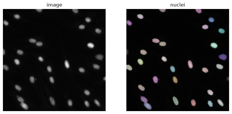

What does StarDist predict?¶

details holds what the network predicted for each object:

points: the centre of each object
coord: the end points of the rays, which together form the polygon outline
prob: how sure the network is that this is an object

Below we draw the polygons on the image. With show_dist=True the rays from the centre to the boundary are drawn as well.

from stardist import _draw_polygons

fig, axs = plt.subplots(1, 2, figsize=(10, 5))
# Polygons and rays predicted for every nucleus
_ = axs[0].imshow(img_dsb, cmap="gray")
plt.sca(axs[0])  # _draw_polygons draws on the current axes
_draw_polygons(details["coord"], details["points"], details["prob"], show_dist=True)
_ = axs[0].set_title("polygons and rays")
_ = axs[0].axis("off")
# Probability of every detected nucleus
_ = axs[1].hist(details["prob"], bins=20)
_ = axs[1].set_xlabel("probability")
_ = axs[1].set_ylabel("number of nuclei")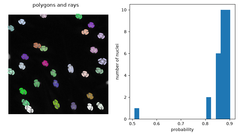

Let’s try with some other images¶

We have a few images from an experiment studying the formation of DNA repair foci in the nucleus after radiations. Cells were either irradiated (IR) or left untreated (control), fixed 2 hours later, and imaged in two channels:

channel 0: DNA damage foci (anti-RAD51 antibody) the bright dots inside the nuclei
channel 1: the nuclei (DAPI)

For now we only use the nuclei channel. We will later try to also detect the foci, where we count how many of them sit in each nucleus.

img = tiff.imread("data/MAX_2h_IR_Position002.tif")
print(img.shape)

# Split the two channels
img_foci   = img[0, :, :]
img_nuclei = img[1, :, :]

fig, axs = plt.subplots(1, 2, figsize=(10, 5))
_ = axs[0].imshow(img_foci, cmap="gray")
_ = axs[0].set_title("channel 0: foci")
_ = axs[1].imshow(img_nuclei, cmap="gray")
_ = axs[1].set_title("channel 1: nuclei")
for ax in axs:
    _ = ax.axis("off")

(2, 1024, 1024)

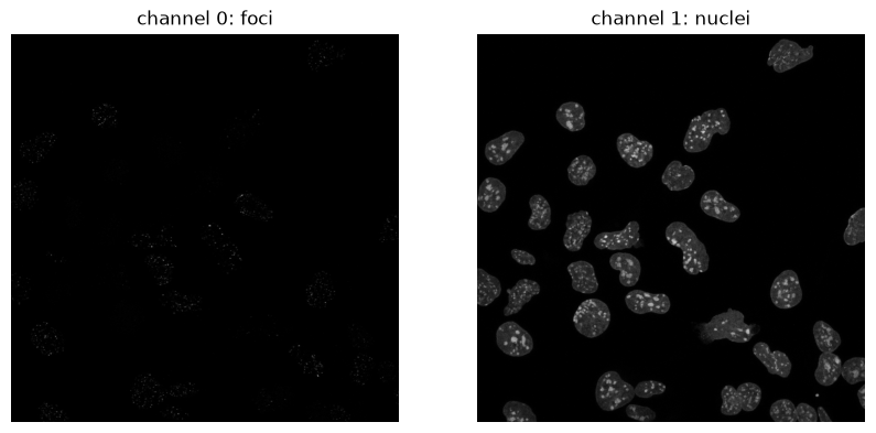
The foci in the first channel are not very clear to see. You could check the maximum intensity in the image with img_foci.max(). Then you could use the argument vmax=50 at imshow() at the right place in the code above to scale the maximum intensity shown.

A first attempt¶

Let us do exactly what we did before: normalize, then predict.

img_nuclei_norm = normalize(img_nuclei, 1, 99.8)

labels_naive, _ = model.predict_instances(img_nuclei_norm)
print(f"found {labels_naive.max()} nuclei")

_ = plt.figure(figsize=(7, 7))
_ = plt.imshow(img_nuclei, cmap="gray")
_ = plt.imshow(labels_naive, cmap=lbl_cmap, alpha=0.5)
_ = plt.title(f"{labels_naive.max()} objects")
_ = plt.axis("off")

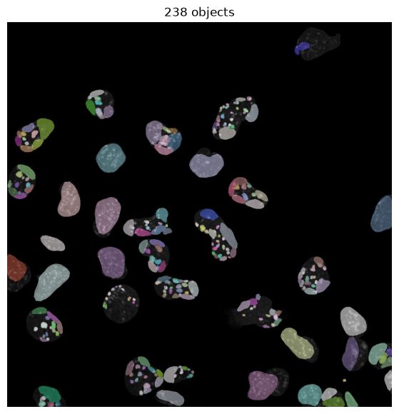
found 238 nuclei

Improving the result¶

That is far too many objects, the results show that single nuclei are cut into several pieces.

The reason is the size of the nuclei. The network learned what a nucleus looks like at the pixel size of its training images. In the example image above the nuclei are about 15 pixels across. Our nuclei are around 80 pixels across. Inside the nuclei are nucleoli and those are more the size the model expects.

So we will show the image to the network at a smaller scale. predict_instances() has a scale argument for this: it downscales the image, predicts, and converts the labels back onto the original pixel grid, so labels has the same shape as the input image.

labels, details = model.predict_instances(img_nuclei_norm, scale=0.5)

print(f"found {labels.max()} nuclei")
print(f"label image shape: {labels.shape}  (same as the input: {img_nuclei.shape})")

found 38 nuclei
label image shape: (1024, 1024)  (same as the input: (1024, 1024))

fig, axs = plt.subplots(1, 2, figsize=(12, 6))
# Prediction at the original scale
_ = axs[0].imshow(img_nuclei, cmap="gray")
_ = axs[0].imshow(labels_naive, cmap=lbl_cmap, alpha=0.5)
_ = axs[0].set_title(f"scale=1 (default): {labels_naive.max()} objects")
# Prediction on the downscaled image
_ = axs[1].imshow(img_nuclei, cmap="gray")
_ = axs[1].imshow(labels, cmap=lbl_cmap, alpha=0.5)
_ = axs[1].set_title(f"scale=0.5: {labels.max()} objects")
for ax in axs:
    _ = ax.axis("off")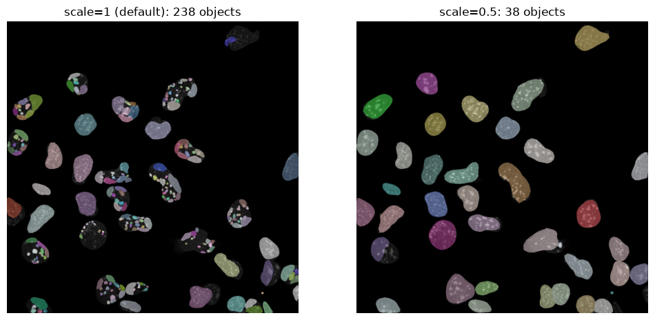

Exercise: What happens if you do not normalize?¶

Run predict_instances() on img_nuclei without normalizing it first (keep scale=0.5), and plot the result next to the normalized one.

How many objects do you get?
Which objects did it find instead of the nuclei?

Exercise: Which scale works best?¶

We picked scale=0.5 without checking. Try a few values (for example 0.25, 0.4, 0.5, 0.75). You could try and plot the number of detected objects against the scale.

Which scale gives a sensible result in the overlay?
You could try to load another image of the data set and check that image as well.

Next¶

We now have nuclei as a label image. In the next notebook we do the same job with Cellpose, which uses a different trick to find objects and asks for the object size in a different way.

Extra: multiplex image¶

Here we explore how to use StarDist on large 2D images. For example with this multiplex image provided as example in the QuPath software.

Download the file LuCa-7color_[13860,52919]_1x1component_data.tif from https://downloads.openmicroscopy.org/images/Vectra-QPTIFF/perkinelmer/PKI_fields/ Save it in the data folder.

luca = tiff.imread("data/LuCa-7color_[13860,52919]_1x1component_data.tif")
print(luca.shape)

(8, 1400, 1868)

channel_names = [
    "PDL1", "CD8", "FoxP3", "CD68",
    "PD1", "CK", "DAPI", "Auto-fluorescence"
]

fig, axs = plt.subplots(2, 4, figsize=(12, 6))
axs = axs.ravel()

for channel, marker in enumerate(channel_names):
    axs[channel].imshow(
        luca[channel, ...], # looking at the shape of the luca array, we see that the first dimension is the channel dimension, so we index it with i to get the ith channel
        cmap="gray",
        vmax=np.percentile(luca[channel, ...], 99.5)
    )
    axs[channel].set_title(f"channel {channel}: {name}")
    axs[channel].axis("off")

plt.tight_layout()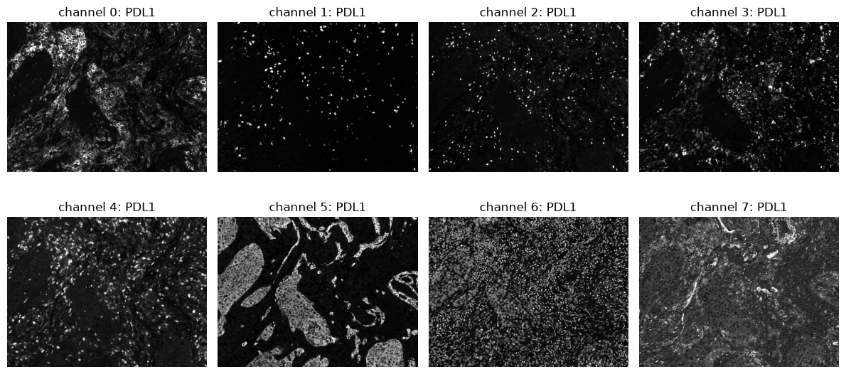

Running stardist or any other AI model on large images (either 2D or 3D) can consume a lot more computer memory and often cannot be done at once. We can therefore split the image up into pieces. We create the label maps of the separate ‘tiles’ with some overlap and put them together again in the end. In StarDist this is done with the n_tiles argument.

# Channel 6 is the nuclear stain (DAPI)
nuclei_luca = luca[6, ...]
nuclei_luca_norm = normalize(nuclei_luca, 1, 99.8)

labels_luca, details = model.predict_instances(nuclei_luca_norm, n_tiles=(4, 4))

100%|█████████████████████████████████████████████████████████████| 16/16 [00:02<00:00,  5.36it/s]

#Let's visualize the results.
fig, axs = plt.subplots(1, 2, figsize=(20, 10))
# The raw image
_ = axs[0].imshow(nuclei_luca, cmap="gray")
_ = axs[0].set_title("image")
# The same image with the labels on top
_ = axs[1].imshow(nuclei_luca, cmap="gray")
_ = axs[1].imshow(labels_luca, cmap=lbl_cmap, alpha=0.5)
_ = axs[1].set_title("nuclei")
for ax in axs:
    _ = ax.axis("off")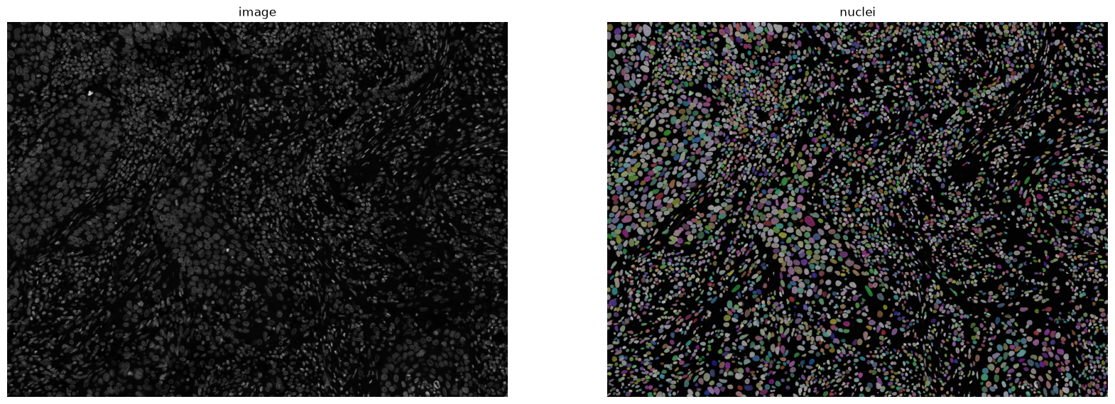

As you can see some of the proteins in the channels above are in the cytoplasm. If we want to measure the intensity in the cytoplasm we can use label expansion: we grow each label by a certain distance, or until it touches another cell. scikit-image has a function for this called expand_labels(). Then we remove the nucleus from each expanded label, so only a ring of cytoplasm around each nucleus is left.

# Expand the labels by 10 pixels
from skimage.segmentation import expand_labels
expanded_labels_luca = expand_labels(labels_luca, distance=10)

# Keep the expanded labels only where there is no nucleus: a ring of cytoplasm
cytoplasm_mask = np.where(labels_luca > 0, 0, expanded_labels_luca)

#Let's visualize the results.
fig, axs = plt.subplots(1, 2, figsize=(20, 10))
# The raw image
_ = axs[0].imshow(nuclei_luca, cmap="gray")
_ = axs[0].set_title("image")
# The same image with the cytoplasm labels on top
_ = axs[1].imshow(nuclei_luca, cmap="gray")
_ = axs[1].imshow(cytoplasm_mask, cmap=lbl_cmap, alpha=0.3)
_ = axs[1].set_title("cytoplasm")
for ax in axs:
    _ = ax.axis("off")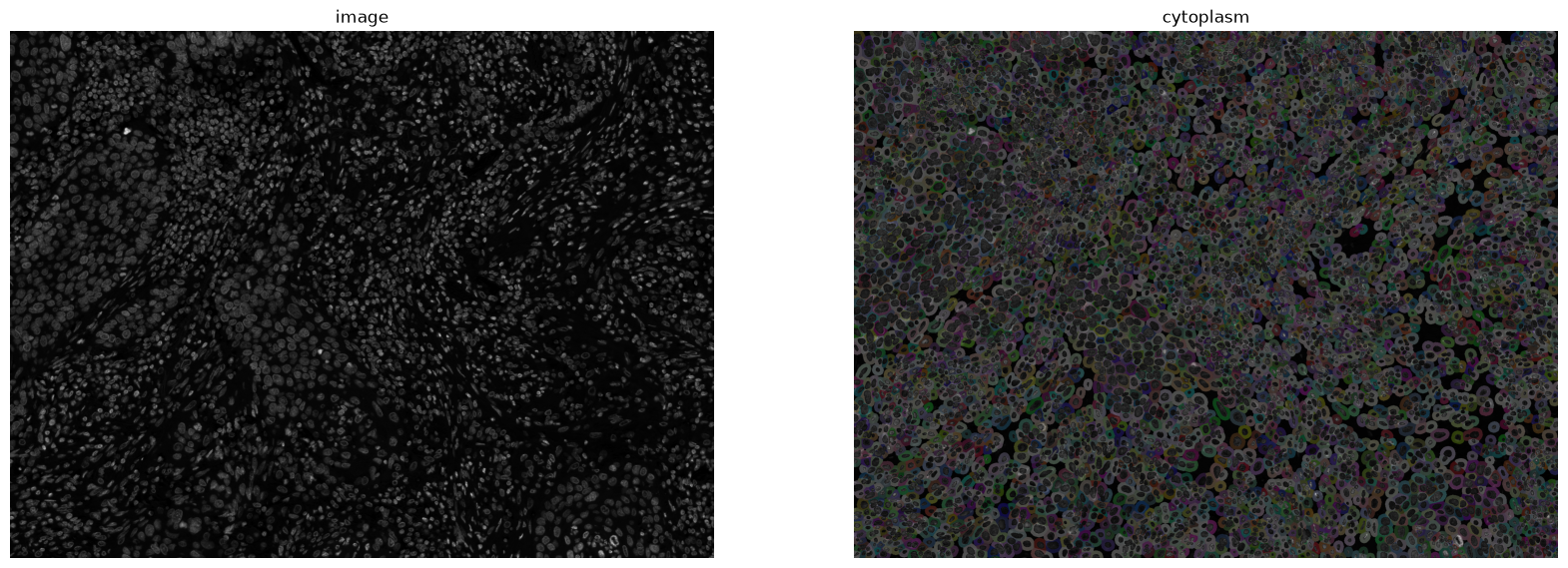

# Measure marker intensities in the cytoplasm ring around each nucleus
marker_measurements = {}

for channel, marker in enumerate(channel_names):
    props = sk.measure.regionprops_table(
        cytoplasm_mask,
        intensity_image=luca[channel],
        properties=("label", "area", "intensity_mean", "intensity_max"),
    )
    marker_measurements[marker] = props

# Plot the distribution of mean marker intensities per cell
fig, axs = plt.subplots(2, 4, figsize=(16, 8))
axs = axs.ravel()

for ax, marker in zip(axs, channel_names):
    values = marker_measurements[marker]["intensity_mean"]
    ax.hist(values, bins=50, color="steelblue", alpha=0.8)
    ax.set_title(marker)
    ax.set_xlabel("Mean intensity in cytoplasm per cell")
    ax.set_ylabel("Number of cytoplasm regions")
    ax.set_yscale("log")

plt.tight_layout()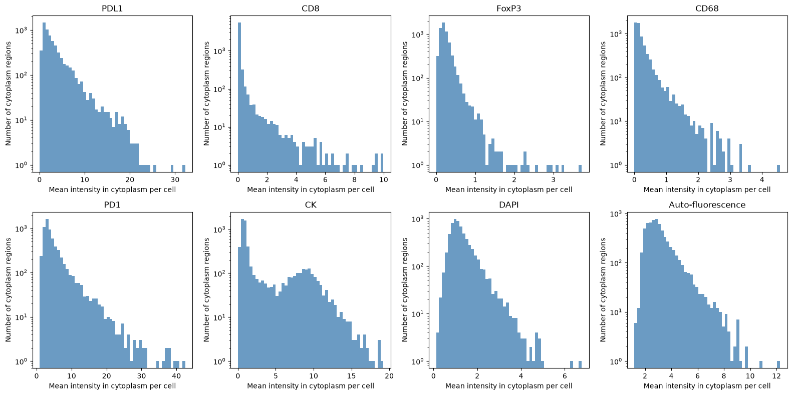

Note: If you would like to explore this further you could also download an H&E image from the link above. StarDist also has a model that can segment nuclei from brightfield images.

This analysis is done with an image of 80 MB, however when images get much larger we should think of ways to not store all data in the computer memory at once, for example by storing data in OME-zarr format. This helps to only read the part of the data that we need at that moment or using the dask library to manage the loading of the data in an efficient way.

Here is a notebook that shows these options: examples/other2D/predict_big_data.ipynb

3D? StarDist also has models for 3D data. You can explore the possibilities here: https://github.com/stardist/stardist/tree/main/examples